Beautiful plots while simulating loss in two-part procrustes problem

14Apr15

Today I was working on a two-part procrustes problem and wanted to find out why my minimization algorithm sometimes does not converge properly or renders unexpected results. The loss function to be minimized is

$\displaystyle L(\mathbf{Q},c) = \| c \mathbf{A_1Q} - \mathbf{B_1} \|^2 + \| \mathbf{A_2Q} - \mathbf{B_2} \|^2 \rightarrow min$

with $\| \cdot \|$ denoting the Frobenius norm, $c$ is an unknown scalar and $\mathbf{Q}$ an unknown rotation matrix, i.e. $\mathbf{Q}^T\mathbf{Q}=\mathbf{I}$ . $\;\mathbf{A_1}, \mathbf{A_2}, \mathbf{B_1}$ , and $\mathbf{B_1}$ are four real valued matrices. The minimum for $c$ is easily found by setting the partial derivation of $L(\mathbf{Q},c)$ w.r.t $c$ equal to zero.

$\displaystyle c = \frac {tr \; \mathbf{Q}^T \mathbf{A_1}^T \mathbf{B_1}} { \| \mathbf{A_1} \|^2 }$

By plugging $c$ into the loss function $L(\mathbf{Q},c)$ we get a new loss function $L(\mathbf{Q})$ that only depends on $\mathbf{Q}$ . This is the starting situation.

When trying to find out why the algorithm to minimize $L(\mathbf{Q})$ did not work as expected, I got stuck. So I decided to conduct a small simulation and generate random rotation matrices to study the relation between the parameter $c$ and the value of the loss function $L(\mathbf{Q})$ . Before looking at the results for the entire two-part procrustes problem from above, let’s visualize the results for the first part of the loss function only, i.e.

$\displaystyle L(\mathbf{Q},c) = \| c \mathbf{A_1Q} - \mathbf{B_1} \|^2 \rightarrow min$

Here, $c$ has the same minimum as for the whole formula above. For the simulation I used

$\mathbf{A_1}= \begin{pmatrix} 0.0 & 0.4 & -0.5 \\ -0.4 & -0.8 & -0.5 \\ -0.1 & -0.5 & 0.2 \\ \end{pmatrix} \mkern18mu \qquad \text{and} \qquad \mkern36mu \mathbf{B_1}= \begin{pmatrix} -0.1 & -0.8 & -0.1 \\ 0.3 & 0.2 & -0.9 \\ 0.1 & -0.3 & -0.5 \\ \end{pmatrix}$

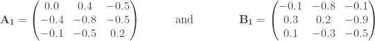
as input matrices. Generating many random rotation matrices $\mathbf{Q}$ and plotting $c$ against the value of the loss function yields the following plot.

This is a well behaved relation, for each scaling parameter $c$ the loss is identical. Now let’s look at the full two-part loss function. As input matrices I used

$\displaystyle A1= \begin{pmatrix} 0.0 & 0.4 & -0.5 \\ -0.4 & -0.8 & -0.5 \\ -0.1 & -0.5 & 0.2 \\ \end{pmatrix} \mkern18mu , \mkern36mu B1= \begin{pmatrix} -0.1 & -0.8 & -0.1 \\ 0.3 & 0.2 & -0.9 \\ 0.1 & -0.3 & -0.5 \\ \end{pmatrix}$
$A2= \begin{pmatrix} 0 & 0 & 1 \\ 1 & 0 & 0 \\ 0 & 1 & 0 \\ \end{pmatrix} \mkern18mu , \mkern36mu B2= \begin{pmatrix} 0 & 0 & 1 \\ 1 & 0 & 0 \\ 0 & 1 & 0 \\ \end{pmatrix}$

and the following R-code.

# trace function
tr <- function(X) sum(diag(X))

# random matrix type 1
rmat_1 <- function(n=3, p=3, min=-1, max=1){
  matrix(runif(n*p, min, max), ncol=p)
}

# random matrix type 2, sparse
rmat_2 <- function(p=3) {
  diag(p)[, sample(1:p, p)]
}

# generate random rotation matrix Q. Based on Q find 
# optimal scaling factor c and calculate loss function value
#
one_sample <- function(n=2, p=2)
{
  Q <- mixAK::rRotationMatrix(n=1, dim=p) %*%         # random rotation matrix det(Q) = 1
    diag(sample(c(-1,1), p, rep=T))                   # additional reflections, so det(Q) in {-1,1}
  s <- tr( t(Q) %*% t(A1) %*% B1 ) / norm(A1, "F")^2  # scaling factor c
  rss <- norm(s*A1 %*% Q - B1, "F")^2 +               # get residual sum of squares
         norm(A2 %*% Q - B2, "F")^2 
  c(s=s, rss=rss)
}

# find c and rss or many random rotation matrices
#
set.seed(10)  # nice case for 3 x 3
n <- 3
p <- 3
A1 <- round(rmat_1(n, p), 1)
B1 <- round(rmat_1(n, p), 1)
A2 <- rmat_2(p)
B2 <- rmat_2(p)

x <- plyr::rdply(40000, one_sample(3,3)) 
plot(x$s, x$rss, pch=16, cex=.4, xlab="c", ylab="L(Q)", col="#00000010")

This time the result turns out to be very different and … beautiful :)

Here, we do not have a one to one relation between the scaling parameter and the loss function any more. I do not quite know what to make of this yet. But for now I am happy that it has aestethic value. Below you find some more beautiful graphics with different matrices as inputs.

Cheers!

Filed under: R / R-Code | 4 Comments

4 Responses to “Beautiful plots while simulating loss in two-part procrustes problem”

Feed for this Entry Trackback Address

1 Eric Melse on April 15, 2015 said:

Hi Mark, I try to run your syntax but R returns an error: could not find function “rdply”
So, probably one or more packages are required. If so, which are these?
Regards,
Eric
2 markheckmann on April 15, 2015 said:

Hi Eric, you must load the ‘plyr’ package. I fixed it in the code. Thanks.
3 therrookie on July 15, 2015 said:

Hi Mark, I’m Brand new to R and just started blogging about it as well to help me remember/learn it. Thanks for your blog. Is there a contact page on your wordpress site? I couldn’t find one.

I found you R Google search blog incredibly helpful, and had a question, but i think the comments were closed. https://ryouready.wordpress.com/2009/01/01/r-retrieving-information-from-google-with-rcurl-package/.

I recently used it to grab all locations of a particular company across the US. I was curious if there was way to get to page 2 of Google using that code?

Thanks again,
4 markheckmann on July 15, 2015 said:

Hi,
glad that you like the site:) Concerning Google, you can pass the ‘start’ parameter in the GET request, e.g. ‘start=10’ to get the second page. If you are not familiaer with the structure of GET requests, you may want to read about that first..
HTH
Bests
Mark